Quantcast
Channel: SAP Adaptive Server Enterprise (SAP ASE) for Custom Applications
Viewing all 151 articles
Browse latest View live

ASE 15.7: ESD#4 UPDATES….

$
0
0

ESD#4 has been around for some time.  I did not start testing the conditions I am pushing the ASE into with this EBF for several reasons.  But now it seems to really be a pity I haven’t done so from the start.  After making a few tests with ESD#2 on Solaris x64, and after making similar tests with ESD#3 on Solaris SPARC I decided to move on.  The reason for this is that I was not really satisfied with what I saw.  True, I am pushing the ASE into an area which is very imcomfortable for it (simulating a situation which a highly respected Sybase engineer has called running a “really bad code”).  But this is a real-client situation and I must know how my ASE will handle it.  It is really naive to think that ASE should handle only properly formed workload written by developer teams sensitive to the way DB operates.  Today more and more code is written which care very little for DB needs.  Either we face it or the customers moves to DBMS systems that cope with “bad code” better than ASE…

So, on the one hand, I was not satisfied with the results of my tests – especially with high spinlock contention for various spinlocks guarding the procedure / statement cache.  On the other, ESD#4 (and the weird fish ESD#3.1, which has only a little portion of fixes out of ESD#4, but came later on – a couple of days ago in fact) says to have worked on the procedure cache spinlock contention a little more.  Since this is what I was after, I switched the direction a bit.

Unfortunately, I could not spend much time on the current tests, and I will not be able to spend any more time on them in days to come (customer calls).  I did succeed, though, to do some initial tests which I would like to share.  Especially since there is a parallel discussion on ISUG SIG area (now restricted to paid members only) which mentions statement cache issues.  Lovely discussion, but it really deals with how to tune the ASE to handle “good code” without waste of resources and how to monitor the waste.  It still avoids the situation when the ASE is bombarded with “bad code.”

An aside installation note on ESD#4.  I had to truss the installation process since it has been constantly hanging.  As it turned out, the space requirement which the installation checks does not take into account available swap space.  Installer uses /tmp quite freely, and my 800MB of /tmp was not enough for the installation of this ESD.  Had the installation informed me on this requirement in time, it might have saved me some time and pain.  I hope the good code that manages the installation will be made even better in future…

So here are the settings:

ESD#209:3009:3509:4009:4309:4509:5009:5510:0010:03
STREAM011101011
PLAN SH001100001
STCACHE(J)000011111
DYNPREP(J)111111111
STCACHE(MB)000202020202020


ESD#2
10:0610:1210:1510:2010:2310:2510:2810:30
STREAM
11001111
PLAN SH
10000111
STCACHE(J)
11111111
DYNPREP(J)
11101000
STCACHE(MB)
10010010010010010020100


ESD#412:5612:5812:5913:0113:0213:0313:0413:0613:07
STREAM011101111
PLAN SH001100110
STCACHE(J)000011111
DYNPREP(J)111111111
STCACHE(MB)00020202020100100


ESD#4
13:0813:1013:1113:1213:14


STREAM
00111


PLAN SH
00011


STCACHE(J)
11111


DYNPREP(J)
00000


STCACHE(MB)
10010010010020


Really what it says is that we are playing with 3 DB and 2 JDBC client options.  On the DB side we are playing with streamlined dynamic SQL, plan sharing and statement cache size.  On the JDBC client side we are playing with DYNAMIC_PREPARED and set statement_cache on setting (the last is not really on JDBC side, but addresses the needs of that client).  Our aim:  to keep ASE from crumbling beneath the bad code, which in the time before statement cache refinements was manageable.

We start with ESD#2

1CPU

Statement Cache situation:

1ST_CACHE

Spinlock situation:

1SPINS

The rate of LWP/Dynamic SQLs creation:
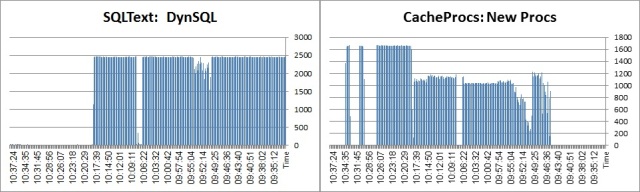
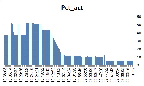
1LWPs

monitorconfig:

1MONCONFIG

Now ESD#4:

CPU

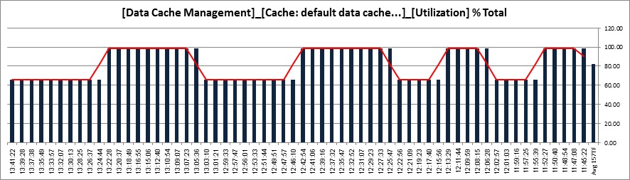
Statemet Cache situation:
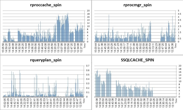
ST_CACHE

Spinlock Situation:

SPINS

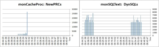
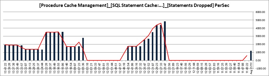
The rate of LWPs/Dynamic SQL creation:

LWPs

monitorconfig

PROC_MON

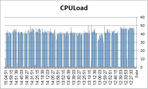
Before anything else, I must add a short note about reducing the size of statement cache.  Although the configuration parameter is dynamic, both in ESD#2 and ESD#4 there is a real problem reducing its size.  After the statement cache has been utilized (100 MB in my tests), when the statement cache is reduced to a lower value (20 MB or even 0 MB) the memory is not released.  This causes a sensible spike in CPU utilization   and a large SSQLCACHE spinlock contention seen on the graphs above.  Probably a bug.   This is what prsqlcache reports:

1> sp_configure “statement cache”, 0
2> go
Parameter Name Default Memory Used Config Value Run Value Unit Type
———— ——————– ———– ——————– ——————– ——————– ——————–
statement cache size 0 0 0 0 memory pages(2k) dynamic

(1 row affected)
Configuration option changed. ASE need not be rebooted since the option is dynamic.
Changing the value of ‘statement cache size’ does not increase the amount of memory Adaptive Server uses.
(return status = 0)

1> dbcc prsqlcache
2> go

Start of SSQL Hash Table at 0xfffffd7f4890e050

Memory configured: 0 2k pages Memory used: 35635 2k pages

End of SSQL Hash Table

DBCC execution completed. If DBCC printed error messages, contact a user with System Administrator (SA) role.
1>

Now to the rest of the findings.  It seems that ESD#4 treats the situation of a client code wasting its statement (and procedure) cache memory structures – uselessly turning over the pages chain – much better.  I did not post the data from my tests on a large SPARC host as promised earlier since they were not really better.    With this new information, I will have to rerun the tests next Sunday on the ESD#4, SPARC.  Hopefully, I will get a much improved performance metrics there as well.  I am eager to see the statement cache/procedure cache saga in ASE 15.x to be laid to rest.  It has really been a pain in the neck dealing with this stuff.  I hope that at last we may sigh a relief…  and get back to the optimizer issues….

Next update will probably come on Monday, unless something interesting is discovered before that (and I have time to test and testify on it here).

Yours.

ATM.


ASE 15.7 ESD#4 ON SPARC…

$
0
0

I have just finished the first round of tests of ESD#4 on Solaris SPARC platform.  I have to confirm:  the ESD#4 seems to has been finally vaccinated against wasteful reuse of the statement/procedure cache by “inappropriate” use in client-side code.  It looks like the painful experience of seeing ASE suffocating unexpectedly under the stress generated by the code that has been running “more or less smoothly” on an old ASE 12.5.4 is behind us.  I will cross test these issues again tomorrow (as well as shift my tests a bit to check yet another issue around the misuse of the statement cache).  But so far I must say that I found that ASE handles this situation successfully at last.  Very good news!

Here are the bare facts, again.

The tests I have run on the SPARC host on ASE 12.5.4 version (ESD#10):

S125_6LWP_DYN1_ST0_ST0M_108:50:00
S125_6LWP_DYN0_ST0_ST0M_109:01:00
S125_6LWP_DYN0_ST0_ST20M_109:12:00
S125_6LWP_DYN0_ST1_ST20M_109:22:00
S125_6LWP_DYN1_ST1_ST20M_109:34:00

The tests I have run on the SPARC host on ASE 15.7 – threaded mode kernel (ESD#4):

S157T_6LWP_DYN1_ST0_STR0_PLA0_ST0M_108:50:00
S157T_6LWP_DYN1_ST0_STR1_PLA0_ST0M_109:01:00
S157T_6LWP_DYN1_ST0_STR1_PLA1_ST0M_109:12:00
S157T_6LWP_DYN0_ST0_STR0_PLA0_ST0M_109:22:00
S157T_6LWP_DYN0_ST0_STR1_PLA0_ST0M_109:34:00
S157T_6LWP_DYN0_ST0_STR1_PLA1_ST0M_109:46:00
S157T_6LWP_DYN1_ST0_STR0_PLA0_ST20M_109:56:00
S157T_6LWP_DYN1_ST0_STR1_PLA0_ST20M_110:06:00
S157T_6LWP_DYN1_ST1_STR0_PLA0_ST20M_110:15:00
S157T_6LWP_DYN1_ST1_STR1_PLA0_ST20M_110:24:00
S157T_6LWP_DYN1_ST1_STR1_PLA1_ST20M_110:34:00
S157T_6LWP_DYN0_ST1_STR0_PLA0_ST20M_110:43:00
S157T_6LWP_DYN0_ST1_STR1_PLA0_ST20M_110:52:00
S157T_6LWP_DYN0_ST1_STR1_PLA1_ST20M_111:01:00
S157T_6LWP_DYN0_ST1_STR1_PLA1_ST200M_111:09:00
S157T_6LWP_DYN1_ST1_STR1_PLA1_ST200M_111:17:00

The tests I have run on the SPARC host on ASE 15.7 – process mode kernel (ESD#4):

S157P_6LWP_DYN1_ST0_STR0_PLA0_ST0M_112:24:00
S157P_6LWP_DYN1_ST0_STR1_PLA0_ST0M_112:32:00
S157P_6LWP_DYN1_ST0_STR1_PLA1_ST0M_112:43:00
S157P_6LWP_DYN0_ST0_STR0_PLA0_ST0M_112:52:00
S157P_6LWP_DYN0_ST0_STR1_PLA0_ST0M_113:01:00
S157P_6LWP_DYN0_ST0_STR1_PLA1_ST0M_113:09:00
S157P_6LWP_DYN1_ST0_STR0_PLA0_ST20M_113:18:00
S157P_6LWP_DYN1_ST0_STR1_PLA0_ST20M_113:27:00
S157P_6LWP_DYN1_ST1_STR0_PLA0_ST20M_113:37:00
S157P_6LWP_DYN1_ST1_STR1_PLA0_ST20M_113:45:00
S157P_6LWP_DYN1_ST1_STR1_PLA1_ST20M_113:53:00
S157P_6LWP_DYN0_ST1_STR0_PLA0_ST20M_114:02:00
S157P_6LWP_DYN0_ST1_STR1_PLA0_ST20M_114:11:00
S157P_6LWP_DYN0_ST1_STR1_PLA1_ST20M_114:20:00
S157P_6LWP_DYN0_ST1_STR0_PLA1_ST200M_114:28:00
S157P_6LWP_DYN1_ST1_STR0_PLA1_ST200M_114:37:00
S157P_6LWP_DYN1_ST1_STR1_PLA1_ST200M_114:44:00
S157P_6LWP_DYN0_ST1_STR1_PLA1_ST200M_114:50:00

The performance graphs:

ASE 12.5.4:

CPULOAD

Spinlock Situation (note the way 12.5.4 handles the situation with the statement cache enabled – pure disaster):

SPINS

Procedure Cache:

PCACHE

Dynamic SQL/LWPs creation rate:

LWPS

ASE 15.7 ESD#4 – threaded kernel mode:

Thread Load:

CPULOAD

Spinlock situation:

SPINS

Procedure cache:

PCACHE

Dynamic SQL/LWPs creation rate:

LWPs

Statement Cache (not available on 12.5.4):

STCACHE

ASE 15.7 ESD#4 – process kernel mode:

Engine Load:

CPULOAD

Spinlock situation:

SPINS

Procedure cache:

PCACHE

Dynamic SQL/LWPs creation rate:

LWPs

Statement Cache (not available on 12.5.4):

STCACHE

Threaded kernel mode gives a very steady throughput.  More steady than the process kernel mode.  There is the same “bug” in the process mode that the sp_monitorconfig at certain point stops reporting on procedure cache utilization (I wonder if the new monMemoryUsage MDA supplements the missing data).

In general, if you do have a client that generates a large number of fully prepared statements, DON’Tturn off the statement cache on the session level and DON’T turn off the DYNAMIC_PREPARE JDBC setting.  In both cases, the thread utilization climbs up (and the proccache spinlock).  In addition, if the statement cache us ruthlessly turned over due to very high volume of unique statements generated by the code, keep the cache as small as possible – 20M was fine here, 200M was pretty bad.

The threaded kernel mode gives more satisfactory results – more steady performance, slightly better throughput and less bugs.

I will be running more and different tests in the following weeks – as well as comparing performance across a wider spectrum of metrics – but from the point of view of running a high volume of unique prepared statements the problem of ASE 15.x seems to have been solved at last.

ATM.

All previous forums rolled into this one?

$
0
0

Do I understand this correctly?

All previous forums for ASE, RepSvr, Tuning, etc are now in this one forum?

And since I don't see any historic entries, I assume we will loose all the info contained in the old forums?


Thx,

rick_806

ASE 15.7 ESD#4 Unix Domain Sockets

$
0
0

In the past few days, I have fired up a copy of ASE 15.7ESD#4  to try the new feature Unix Domain Sockets.  I found only a few notes about this feature. The CR listing is source of my information.  CR 667751 has all of the public information that I have found to date.


Here is the heart of the information.


"master afunix unused //<hostname>/<pipe>"


After many failed attempts, I realized how simple this could be.

The ASE Server creates a socket file at start-up based on the master entry in the interfaces file.

In order for this to work, the ASE dataserver must have write access to a folder.

Hmmm-- $SYBASE sounds like a good choice.


I decided I wanted my socket file to be called "ASE.socket" in /sybase/ folder.


Here is an example of the master line that finally worked.


master afunix unused //mytesthost/sybase/ASE.socket


I tested the socket with isql & bcp... Both tools worked without a problem.  The feature of the new connection is to reduce the overhead associated with TCP/IP.  The results of my bcp inbound testing proved that the network layer was not my source of contention and slowness.  I expect that bcp outbound will show better results if I can get past other self-inflicted issues of my machine.


In conclusion, ASE Unix Domain Sockets works without issues when I use the ASE utilities.


ASE 15.7: Prepared Statements and ASE Statement/Procedure Cache, Configuration Impact

$
0
0

So we are back with the same issue:   statement cache/procedure cache behavior under the stress of executing a high volume of prepared statements.  


I have just finished another round of tests around this issue (which has caused quite a lot of troubles in the past releases of ASE) and I want to share and recapitulate (the more you explain the more you understand yourself).


First, let's quote a bit of documentation - to lay out who are the players in our field.  I will reserve it to a very few aspect of what is relevant.  .


[1] Procedure Cache:  {Performance and Tuning Series: Basics. Chapter 5: Memory Use and Performance}

Adaptive Server maintains an MRU/LRU (most recently used/least recently used) chain of stored procedure query plans.  As users execute stored procedures, Adaptive Server looks in the procedure cache for a query plan to use.  If a query plan is available, it is placed on the MRU end of the chain, and execution begins.

...

The memory allocated for the procedure cache holds the optimized query plans (and occasionally trees) for all batches, including any triggers.


[2] Statement Cache:  {Performance and Tuning Series: Basics. Chapter 5: Memory Use and Performance}

The statement cache saves SQL text and plans previously generated for ad hoc SQL statements, enabling Adaptive Server to avoid recompiling incoming SQL that matches a previously cached statement. When enabled, the statement cache reserves a portion of the procedure cache


[3] Streamlined Dynamic SQL:  {Performance and Tuning Series: Basics. Chapter 5: Memory Use and Performance}

In versions earlier than 15.7, Adaptive Server stored dynamic SQL statements (prepared statements) and their corresponding LWP in the dynamic SQL cache.  Each LWP for a dynamic SQL statement was identified based on the connection metadata.  Because connections had different LWPs associated with the same SQL statement, they could not reuse or share the same LWP.  In addition, all LWPS and query plans created by the connection were lost when the Dynamic SQL cache was released.

In versions 15.7 and later, Adaptive Server uses the statement cache to also store dynamic SQL statements converted to LWPs.  Because the statement cache is shared among all connections, dynamic SQL statements can be reused across connections.


[4] DYNAMIC_PREPARE property:

When client connection executing prepared statement sends request to ASE, it may either send language command as plain SQL text (if DYNP is set to false), or request an ASE to create LWP for it (if DYNP is set to true - something that may be seen in monSysSQLText as "create proc dynXXX as..." & DYNAMIC_SQL dynXXX...).

To quote from Managing Workloads with ASE, "The statement cache reproduces the same benefits as fully prepared statements as it takes language commands from client applications, replaces literals with parameters, creates a statement hash key, compiles and optimizes the statement, and creates a Light Weight Proc for re‐use."


In plain language, we may describe the playground of our tests in the following way:


When a client connection sends an ASE a request, if this request contains a prepared statement, the client connection will either send it as it is (SQLLANG) or convert it into a create procedure request (DYNP/LWP). If the statement cache is enabled on ASE, ASE will store the SQL text & pointer to its LWP in the statement cache, install the plan/tree of the corresponding LWP in the procedure cache and ultimately execute it.


The motivation behind all this is to reuse as much resources within ASE as possible. Without the statement cache, each adhoc query has to be "converted" [parsed/normalized/compiled] into query plan individually and dropped after being executed, thus preventing reuse. With statement cache enabled, the query is looked up in the statement cache instead and if the match is found its plan is cloned from the procedure cache and executed.  If it is not there, it will be  "converted" and installed for reuse.


The same applies to prepared statement. Without the statement cache [and when streamlined option is turned off], each prepared statement has to be converted [parsed/normalized/compiled] into query plan and stored in the procedure cache individually - to be released at client disconnect. With statement cache and streamlined option enabled, the statement is looked up, cloned and executed (or stored for later reuse).


In fact, this "reuse" methodology is a patented feature [2012]. It involves scanning statement/procedure cache memory page chains (holding spinlock) and either installing a new or reusing an old object.


StCacheSearch


In fact, one may collect quite a lot of information on all this over the web.


So far the theory.   We know who is the player on our testing grounds.  What we will see below based on the tests done is how ASE reacts to changing different configuration parameters related to the relatively new aggressive resource reuse aim.

I have confined myself in the tests to only four possible setting to play with:  existence of the statement cache (STxM), streamlined SQL option (STRx), DYNAMIC_PREPARE option (DYNPx) and configuring connection setting to use statement_cache (STx). This results in the following matrix of possible tests:


pst_TestTimes


I run 10 Java clients executing unique prepared statements on a 15-thread ASE, 15.7 ESD#4, SPARC.  The "literal autoparam" setting is turned on, so is the "plan sharing" option.


The first graph represents the thread busy for all our tests:


pst_ThreadBusy


First thing to notice is that whenever the prepared statement meets an ASE, if the connection property of DYNAMIC_PREPARE is turned off, ASE responds in 5 to 10 % leap in thread utilization.  On the one hand, it seems pretty obvious:  we "reuse" LWPs rather than demand ASE to generate (parse/normalize/compile) plan for each statement over and over again.  This is no so obvious, though, since in our case we generate LWPs wrapping 10 completely unique streams of prepared statements.  Reuse here is pretty minimal.  It seems a bit odd that making an ASE to scan its statement cache, install new LWP + QP and execute it to have less CPU impact than just prepare the plan and drop it.  The numbers, though, are unequivocal.   Even if ASE faces a thick stream of unique prepared statements requests, it handles it much better if the client requests them as procedures (incidentally, it was NOT the case with previous ASE 15 releases).


I'd like to share also the following graph:


pst_OpenObjects


We know from documentation that each cached statement consumes one object descriptor.  So it makes sense that turning the statement cache on the number of active object descriptors will rise [12:25].  The impact, though, is much greater when the streamlined option is turned on.  Something to be kept in mind.


This one is also interesting:


pst_LockRequests

pst_ShraedRow


Each time the DYNP is turned on, the number of lock requests is doubled.


This one is also telling:


pst_TDB_Util

pst_DDC_Util


Since we create our LWPs in tempdb, and since we run exclusively the code that causes ASE to generate LWPs, each time the DYNP is turned on, tempdb utilization surges up.


Now, let's see how we are handling procedure requests and statements requests in each case:


Procedures:

pst_ProcReq

pst_ProcRem


Statements:


pst_StCachedpst_StDroppedpst_StINCachepst_StNotCachedpst_StNotINCache


We run 12K procedure requests per second.  Demand on the statement cache is highest when we run DYNPs streaming them into the statement cache (streamlined on).


Happily enough, this high volume of prepared statements washing the statement/procedure cache is handled with a relatively low spinlock contention (I will test it running client connections > threads situation in future).


pst_SpinPCHpst_SpinPMGRpst_SpinQRYPpst_SpinSSQL


It is important to state here that ASE runs with TF758 turned on.  Without it you would have seen proc_cache spinlock getting to 10-s.


Let's see the statement cache utilization from another angle (monStatementCache):


pst_STCACHE


Our cache hit ratio is not impressive (little wonder in our situation of running unique statements from 10 concurrent sessions).   What is interesting to notice, though, is the number of statement the same 20MB cache contains running with and without the streamlined option.  Turning the streamlined option on caused the number of statements contained in the statement cache to double.


The following displays what the client connection requests from ASE in terms of LWP requests:


pst_DYNSQLS


When we turn the DYNP on we start requesting to create procedure from ASE explicitly.  However, the lifetime of the procedures in the cache is reverse:  when DYNP is off, ASE creates procedures implicitly and stores them in the statement cache + procedure cache.  When DYNP is on, ASE creates the procedure and drops it almost instantly - unless the streamlined option is turned on, causing ASE to store them in the statement cache as well - in a far greater number (incidentally, the names of the DYNP LWPs and ADHOC LWPs also differ).


So, what have we learned from all this, if at all?


From the ASE load perspective, we have seen that configuring the ASE to reuse (streamline) the dynamic SQLs is beneficial even if we face a situation of concurrent client connections generating a high volume of unique prepared statements.  Turning the DYNAMIC_PREPARE option off would only cause an additional 10% surge in CPU utilization (there is a problem that we do not really know how the throughput is influenced but rather assume it from the rate of procedure request, which is not precisely true - I will have to change the way I perform the load in future in order to generate more accurate comparison here).


We have learned that forcing ASE to reuse (streamline) the dynamic SQLs will force the procedure cache to handle much more plans/trees since in addition to adhoc queries landing in the statement/procedure cache to aged out, LWPs and their plans that would have died as clients disconnect will continue to occupy both statement and procedure cache, until they age out.  Although we have seen that setting the streamlined option on is beneficial to an ASE in our situation, we must not neglect this fact (after all we run each test at a time, not mix - had we mixed, both adhocs and dynps would land in the same area).   In addition, since statement cache is a general resource, if we know that we have bad (unique & high volume) DYNPs workload threatening to wash out our statement cache, perhaps the best decision would be to turn the streamlined option off and keep these DYNPs off statement cache altogether.


We have learned that open objects usage surges up with the streamlined option turned on, so it must be addressed in configuration in order to avoid descriptor reuse.


We have learned that we have to treat tempdb differently if we know that we will be streamlining.  It's utilization goes way up when ASE has to create LWPs at high rate, so additional attention is needed here.


What we have not understood is what is the origin of the consistent leap in shared row requests when we configure DYNAMIC_PREPARE to true.  Is it because we handle explicit create procedure requests?   To be tested further.


What we have also learned is how the configurations affecting statement cache may influence the procedure cache.  Documentation states that "statement cache memory is taken from the procedure cache memory pool" - a puzzling statement since the memory consumption of both is added together (logical/physical ASE memory) System Administration Guide: Volume 2, Configuring Memory.  What is obvious, though, is that the two have very high degree of reciprocity:  each statement landing into statement cache will have to consume space in the procedure cache for the LWP tree/plan.  Which means that statement cache is not a portion of  procedure cache.  If configured, it will consume a portion of procedure cache which is directly influenced by its size (it is said to be reserved ahead in the documentation).   This is much more accurate way to explain the relationship between statement cache and procedure cache.


We still know very little about the procedure cache.  We know that it has its chain (one, or more if it has already been implemented) of procedure query plans/trees.  We do not know, for example, which of the procedure cache modules / allocators each occupy and if these have been partitioned.  I did monitor the impact of the tests I run on both, but the data it generated has been pretty confusing/uninformative.  Especially so since there is no documentation whatsoever explaining procedure cache structure in details.  We also know very little about ELC and its impact on our tests - although it is pretty sure that it plays a role here (TF758 may testify this).


Which returns us to a famous Socratic sage:   the more you know the more you know you don't know...


Hm,  should we start the testing over?


ATM.

ASE 15.7: Threaded vs. Process Kernel Mode - Solaris/RHEL cross-tests

$
0
0

I am back with the comparative tests:  threaded kernel mode versus process kernel mode.  I have seen in  my earlier tests that process kernel mode seems to get slightly better throughput under the same workload.  On the other hand, I have also found that process kernel mode have shown certain types of unwanted behavior absent from the threaded kernel mode.


In order to verify these differences I decided to port the tests from the Solaris (SPARC) platform to Redhat Linux (Xeon). This way I will be able to test ASE behavior on different platforms: Solaris running on SPARC and RHEL running on Xeon.  The probability of an error will be minimized.


Having performed identical test, I have indeed been able to verify that the threaded kernel mode displays up to 10% more CPU utilization.  Behavioral lapses in the process mode too were persistent across platforms.


What I will report below is a series of 4 tests. Two of them performed on a SPARC host (32 logical processors) with ASE running in threaded and process mode, and another two performed on a XEON host (32 logical processors) with ASE running again in threaded and process modes.  The legend of the tests is identical to my previous posts, so I will not repeat it here.  I am still working around the issue of generating prepared statements at high rate.


SPARC_TESTS


XEON_TESTS

I will post only a limited number of graphs, those that looked most peculiar to me.  I will not comment on how differences in configurations affected the CPU utilization/throughput either (this too is found in earlier posts).


First the TPS/CPU Load:


SPARC:

TPS.SOL

XEON:

TPS.LX


ProcPS/CPU Load:


SPARC:

PROC_REQ.SOL

PC_MON.pr.solPC_MON.th.sol

XEON:

PROC_REQ.LX

PC_MON.pr.lxPC_MON.th.lx


Statement Cache:


SPARC:

ST_CACHED.SOLST_DROPPED.SOLST_FOUND_IN_CACHE.SOL

XEON:

ST_CACHED.LXST_DROPPED.LXST_FOUND_IN_CACHE.LX


Spinlock Contention:


SPARC:

PCACHE_SPIN.SOLSSQLCACHE_SPIN.SOL

XEON:

PCACHE_SPIN.LXSSQLCACHE_SPIN.LX


There are quite a few interesting things.  The same things were found to be working less well across platforms (such as sp_monitorconfig that stopped reporting utilization at certain time, on either RHEL or SPARC, or PC/SC spinlock contention that were consistently higher in the process mode - even with TF758).  What has been pretty surprising is the huge throughput leap in porting the tests from 8 chip rather old SPARC VI host (16 cores, 32 threads running 2.15 GHz) to 2 chip XEON 2600 host (16 cores, 32 threads running 2.7 GHz).  I will check SPARC VII (2.66 GHz 4-core) and T4 (2.85 GHz 8-core) chips later on to have more data.  But the throughput difference found here is something worth digging into.


Anyway, even with the latest tests there still remained a question:  do we really see greater thread utilization due to a higher throughput that ASE achieves running the threaded mode OR the higher thread utilization brings about a lower throughput instead.  In order to test this I had to modify slightly my tests so that I get more precise recording of the volume of work the server does in each test.


This has brought me to the following numbers (I have tested only the RHEL host - more tests to come):


THROUGHPUT.LX


The 100% utilization corresponds to the threaded kernel mode - we have slightly lower number of code loops (I compare here an average number of loops code in each client connection performs for the same period of time).  The threaded mode gets an average of 240 loops with 100% thread utilization, while the process mode gets 260 loops with 90% engine utilization.  This is not much, but the difference is there.  What is also interesting is the following:


Process Mode:

CODE_LOOPS.pr.lx

Threaded Mode:

CODE_LOOPS.th.lx


Each bar in the graph corresponds to a client connection executing its code (identical).  Whereas in the process kernel mode the throughput deviation between each client may vary (200 to 300!), for the threaded kernel mode this deviation does not exist (within the range of 10 - which is explained by the fact that the threads are activated serially).


So it seems to be true:  the threaded kernel mode does get to a slightly higher thread utilization without an increase in throughput. The difference is not significant, but it is there. On another hand, the threaded mode yields much more stable performance - both in terms of query response time and across many other counters. If I had to choose, I'd choose the threaded kernel mode over the process mode - based on its performance characteristics (probably hosted on Linux - but I have to check this aspect more thoroughly before I comment on it with any degree of reliability).  If you consider that some process mode clients has suffered ~15% drop in throughput in comparison to the threaded mode clients, the 35% improvement other process mode clients received is somewhat compromised.


My last tests before I leave this topic will be focusing on whether the throughput rises when more threads are brought online for the strangled ASE, thus reversing the balance towards the threaded mode.  I will check this across both RHEL and SPARC hosts to have more sanitized data and report on it here.


ATM.

ASE 15.7: Threaded Kernel vs. Process Kernel: Throughput Variance

$
0
0

I have just finished performing a controlled analysis of general performance differences for ASE 15.7 running process and threaded kernel mode on various platforms and hosts (RHEL running on Dell Xeon chips, Solaris running on SPARC M, SPARC T  and x64).  Although there are quite a few differences, the following image tells the story of the throughput variance one may expect when switching between different kernel modes:


PSS_VS_THR_THROUGHPUT


Top to bottom:  the top graph shows response time for the same query run by multiple concurrent client connections (each bar representing an absolute number of query executions a client connection has performed in a period of time - 5 minutes).  Bottom left - an average "throughput" for the client connections running vis-a-vis ASE configured in process kernel mode.  Bottom right - an average "throughput" for the client connections running vis-a-vis ASE configured in threaded kernel mode.   The bottom table(s) describes the type of configuration applied to ASE/JDBC.


The image is a bit bulky, but it is pretty eloquent and consistent - across all the platforms tested.  Even though sometimes it looks like ASE running the process kernel mode out-performs ASE running the threaded kernel mode, if you compare throughput more accurately it becomes clear that threaded kernel mode yields very stable, predictable response time, while the process kernel mode exhibits a bursty, unpredictable response time, with some client sessions outperforming others by as much as 100%.  Performing less controlled tests may create a false impression that the process kernel mode runs faster, which in fact is not really true.


It is nothing new, however.  Predictable response time has been named as one of the aspects the threaded kernel has brought into an ASE.  In the tests I run, both java client sessions and ASE itself were located on the same host, competing for OS resources.  Although there is very little I/O involved in the tests, still there is a telling difference in response time across the kernel modes.


I will not comment on the type of tests run in details here.  The only thing I will say is that you should definitely test your JDBC/ODBC client application with different JDBC/ODBC + ASE settings.  As it may be seen from the throughput variance, configuring ASE/JDBC/ODBC properly does make a difference (although it is not always possible to configure both for the best performance in real-life situation).


Stay curious and check yourself as much as possible...


ATM.

Violin Flash Memory Arrays Certified with SAP Sybase ASE

$
0
0

Violin Memory, Inc., provider of memory-based storage systems, and SAP AG today (April 16th)  announced that Violin 6000 Series Flash Memory Arrays are now certified for interoperability with SAP Sybase Adaptive Server Enterprise (SAP Sybase ASE), delivering reliability and accelerated performance across a range of enterprise applications. Used together, these solutions will provide customers with enhanced and simplified solutions that leverage the power of Violin Flash Memory Arrays and business-critical SAP applications to accelerate transaction-driven environments. Additionally, Violin Memory is now an SAP software solution and technology partner in the SAP PartnerEdge program. It will work with SAP to serve new and existing customers, partners and channels to benefit from solutions from Violin Memory and SAP. Violin products are also available in support of SAP ERP applications.


“The Violin Flash Memory Arrays integrated with SAP Sybase ASE are a key solid-state storage component for the acceleration of business-critical applications from SAP,” said Kevin Ichhpurani, senior vice president, Business Development and Ecosystem Innovation, SAP. “The certification process showed that the arrays can deliver significant performance improvement over traditional disk-based systems, delivering substantial value to customers. In fact, during preliminary internal testing, we have seen 10x improvement in the performance of SAP Sybase ASE running on Violin Flash Memory.”


Read the full story at - http://www.violin-memory.com/news/press-releases/violin-flash-memory-arrays-now-certified-with-sap-sybase-adaptive-server-enterprise-to-accelerate-customer-applications-in-transaction-driven-environments/


ASE FAQ: What do the numbers at the beginning of each line in the errorlog mean?

$
0
0

Q: What do the numbers at the beginning of each line in the errorlog mean?


A: Most entries in the ASE errorlog have a prefix in the form aa:bbbb:ccccc:ddddd:<date> <component> <message>


Example:

00:0000:00000:00001:2013/05/03 08:56:55.35 server  Master device size: 110 megabytes, or 56320 virtual pages. (A virtual page is 2048 bytes.)

00:0000:00000:00001:2013/05/03 08:56:55.37 kernel  Setting console to nonblocking mode.

00:0000:00000:00001:2013/05/03 08:56:55.37 kernel  Console logging is enabled. This is controlled via the 'enable console logging' configuration parameter.


These prefix fields are:


FieldMeaning
aaInstance-id.  This is always 0 for symmetric multiprocessing (SMP) servers, for Cluster Edition (CE) ASE it identifies the instance.
bbbbThread-id (threaded mode) or engine-id (process mode).
cccccFamily thread id (fid).  If the spid is using worker processes to perform parallel processing, this field identifies which one was responsible for the message.
dddddLogical thread id (spid).
dateDate and time the message was generated
componentUsually either <server> or <kernel>, indicates which layer of the ASE code generated the error.  The server layer implements the general database functionality, the kernel layer is the interface to the hardware

Q: Are connections using net password encryption?

$
0
0

Q: Are connections using net password encryption?


Turning on the sp_configure setting “net password encryption required” setting can greatly improve security.  Client applications that have not been programmed to use password encryption send their passwords over then netword in plaintext, where the password can be sniffed.  Turning the “net password encryption required” option on prevents such clients from connecting to ASE (though they will still be sending readable passwords over then network while trying to connect).  Presumably the users will contact the SA asking why they can't connect, allowing the applications to be identified and rewritten to use password encryption.  However, the approach of just turning this option on could cause unacceptable service interruptions.  Is there a way to identify such connections from within ASE before turning on the feature?


A: Yes, assuming the applications have current connections to the server.  It isn’t terribly convenient, but you can run a DBCC PSS(uid,spid) command against a connection. There is a bit set in the field named "p6stat" if net password encryption was not used.


Note: DBCC PSS is not a formally documented command; it's output may change between versions without warning. This example output is from Adaptive Server Enterprise/15.7.0/EBF 20369 SMP ESD#02 /P/Sun_svr4/OS 5.10/ase157esd2/3109/64-bit/FBO/Sat Jul  7 10:07:17 2012


Here I log in without the -X parameter used to turn on net password encryption in ISQL

bret-sun2% isql -Usa -P********
1> select @@spid
2> go

------
     17

(1 row affected)
1> dbcc traceon(3604)
2> go
00:0000:00000:00017:2013/05/03 12:49:27.44 server  DBCC TRACEON 3604, SPID 17
DBCC execution completed. If DBCC printed error messages, contact a user with
System Administrator (SA) role.
1> dbcc pss(1,17)
2> go
{

PSS (any state) for suid 1 - spid 17:

PSS at 0x10006da1a88

PSS Status fields :
pstat=0x10000 (0x00010000 (P_USERPROC))
p2stat=0x1010 (0x00001000 (P2_XLATE), 0x00000010 (P2_DEBUG))
p3stat=0x800 (0x00000800 (P3_PSS_ACTIVE))
p4stat=0x0 (0x00000000)
p5stat=0x8 (0x00000008 (P5_RUSRCONN_USED))
p6stat=0x10 (0x00000010 (P6_NETPWD_NO_ENCRYPT)
p7stat=0x0 (0x00000000)
p8stat=0x0 (0x00000000)
pextstat=0x0 (0x00000000)

In contrast, when net password encryption is used, that bit isn’t set.
In the following example, you can see another bit has been set in p8stat showing which encryption method was used
p8stat=0x2 (0x00000002 (P8_NETPWD_RSA_ENCRYPT3)).
The exact bit set when encryption is used may differ depending on the client and server versions.  For instance, in 15.0.3, the bit set is p6stat=0x40 (0x00000040 (P6_NETPWD_RSA_ENCRYPT)).


bret-sun2% isql -Usa -P******** -X
1> select @@spid
2> go

------
     18

(1 row affected)
1> dbcc traceon(3604)
2> go
00:0000:00000:00018:2013/05/03 12:52:47.79 server  DBCC TRACEON 3604, SPID 18
DBCC execution completed. If DBCC printed error messages, contact a user with
System Administrator (SA) role.
1> dbcc pss(1,18)
2> go
{

PSS (any state) for suid 1 - spid 18:

PSS at 0x10006dba390

PSS Status fields :
pstat=0x10000 (0x00010000 (P_USERPROC))
p2stat=0x1010 (0x00001000 (P2_XLATE), 0x00000010 (P2_DEBUG))
p3stat=0x800 (0x00000800 (P3_PSS_ACTIVE))
p4stat=0x0 (0x00000000)
p5stat=0x8 (0x00000008 (P5_RUSRCONN_USED))
p6stat=0x0 (0x00000000)
p7stat=0x0 (0x00000000)
p8stat=0x2 (0x00000002 (P8_NETPWD_RSA_ENCRYPT3))
pextstat=0x0 (0x00000000)


If you are using ISQL version 15.0 ESD 12 or higher, the new pipe feature can get you the results for every active spid at once.
(my thanks to Dan Thrall for pointing out this improvement to the method).


In this example, the first 14 spids are system processes so don’t have these bits set.
Spid 43 isn’t using network encryption while spid 44 is using it.


1> dbcc pss(0,0)
2> go | egrep "NETPWD|pspid"


pkspid=13434983   pspid=2   pclient_kpid=13434983   parent_spid=2
pkspid=13566056   pspid=3   pclient_kpid=13566056   parent_spid=3
pkspid=13697129   pspid=4   pclient_kpid=13697129   parent_spid=4
pkspid=13828202   pspid=5   pclient_kpid=13828202   parent_spid=5
pkspid=13959275   pspid=6   pclient_kpid=13959275   parent_spid=6
pkspid=14090348   pspid=7   pclient_kpid=14090348   parent_spid=7
pkspid=14221421   pspid=8   pclient_kpid=14221421   parent_spid=8
pkspid=14352494   pspid=9   pclient_kpid=14352494   parent_spid=9
pkspid=14483567   pspid=10   pclient_kpid=14483567   parent_spid=10
pkspid=14614640   pspid=11   pclient_kpid=14614640   parent_spid=11
pkspid=14745713   pspid=12   pclient_kpid=14745713   parent_spid=12
pkspid=14876786   pspid=13   pclient_kpid=14876786   parent_spid=13
pkspid=16711808   pspid=15   pclient_kpid=16711808   parent_spid=15
pkspid=16056443   pspid=20   pclient_kpid=16056443   parent_spid=20
p6stat=0x10 (0x00000010 (P6_NETPWD_NO_ENCRYPT))
pkspid=19071122   pspid=43   pclient_kpid=19071122   parent_spid=43
p8stat=0x2 (0x00000002 (P8_NETPWD_RSA_ENCRYPT3))
pkspid=19202195   pspid=44   pclient_kpid=19202195   parent_spid=44


Capture the contents of master..sysprocesses at the same time so you can correlate the spid with application names, user logins, and ip addresses.


There is an open feature request, CR 700602, to have the pssinfo() function enhanced to be able to output the pstat fields.


Bret Halford

Support Architect, SAP Active Global Support

Sybase, Inc., an SAP Company

385 Interlocken Crescent Suite 300, Broomfield CO 80021, USA

Upgrade Tip - Run DBCC GAM(dbid,0,0,'check') after upgrade to 15.x

$
0
0

Recommendation: After upgrading a pre-15.0 server or database to 15.x, run DBCC GAM(dbid,0,0,'check') as a postupgrade step against each upgraded database.


Why:  To minimize the server downtime for the upgrade, some upgrade steps are deferred to a later time.  Prior to 15.0, extent records on allocation pages contained the slice id for partitioned tables.  The upgrade to 15.0 unpartitions all tables, but the old slice information is left in the extent records.  The extent records with old slice information are subsequently corrected by whatever process first acesses the allocation page after upgrade.


In general, this deferred processing just causes a slight one-time slowing of performance as the extent records are corrected.  However, DBCC CHECKSTORAGE in particular experiences two types of problems the first time it is run after the upgrade (when accessing extent records with the old slice information).  The first is greatly decreased performance, the second is spurious 100016 faults (page not used error). On very large databases, the number of faults reported can be overwhelming.


Sample output with spurious 100016 faults:


1> dbcc checkstorage(testdb)

2> go

Checking testdb: Logical pagesize is 2048 bytes

DBCC CHECKSTORAGE for database 'testdb' sequence 7 completed at April 18 2013

2:33PM. 0 faults and 1777 suspect conditions were located. 0 checks were

aborted. You should investigate the recorded faults, and plan a course of action

that will correct them.

Suspect conditions are to be treated as faults if the same suspect condition

persists in subsequent CHECKSTORAGE operations, or if they are also detected by

other DBCC functions.

1> sp_dbcc_faultreport

2> go


Database Name : testdb


Table Name               Index          PartitionId

         Fault Type

         Page Number

------------------------ -------------- ----------------------------------

         --------------------------------------------------------

         ----------------------------------

test                        0                 32000114

         100025 (row count error)

                      NULL

test                      255                 32000114

         100016 (page not used error)

                       491

test                      255                 32000114

         100016 (page not used error)

                       881

test                      255                 32000114

         100016 (page not used error)

                       887

[snip]


In both cases, the problem is not seen on subsequent executions of CHECKSTORAGE on the same database.  One case with a 120 GB database reported CHECKSTORAGE taking 26 times longer for the first execution than subsequent executions.  CHECKSTORAGE, for reasons as yet unknown, is very inefficient at upgrading the extent records, while DBCC GAM(dbid,0,0,'check') has proven to be the fastest method for upgrading all the extent records.  So I recommend running DBCC GAM after the upgrade, before running DBCC CHECKSTORAGE.  It isn't critical that you do so though, as the problem does clear itself up over time or by the first running of CHECKSTORAGE.


This issue is being tracked under change requests (CR) 681056 (spurious faults)and 632800 (slowness)


About DBCC GAM:


The GAM (Global Allocation Map) is an ASE datastructure used to quickly identify which allocation units have at least one free extent on them.  It is essentially a large bitmap with one bit for each allocation page.  The bit is set on when all 32 extent records are allocated and cleared when less than 32 extent records are allocated.  The 'check' option of DBCC GAM reads each allocation page in the database to verify that the corresponding GAM bit is set correctly.   Prior to ASE 15.7 ESD 4, the 'check' option incorrectly outputs a message saying that the database must be in single user mode.  This message should be ignored as the check is performed regardless.

What is in my statement cache?

$
0
0

I was talking with one of our customers the other day who had a whole bunch of disparate applications attaching to his server.

It really is not unusual from what I have seen to have legacy applications connecting to ASE that the DBA has no knowledge of at all, things just 'work' .


Anyway, from what I explained I thought it would be worth detailing here, there are specific formats and properties of the various entries in

the statement cache that help identify the possible setup of the source application. 

We have enhancements in 15.7 and above to allow dynamic sql to be stored in the regular statement cache also (more on that below).


The statement cache stores the statement text object, the LWPs (lightweight procedures) themselves reside in the procedure cache.


Note that monCachedProcedures\monCachedStatement are the two MDA tables relevant to looking at the individual LWPs.

Here I am making use of of a few things...


show_cached_text(<ssql_id>) --ssql_id being the id of the statement in the statement cache (also the lwp procedure id)

dbcc prsqlcache (<ssql_id>, 0||1) --ssql_id is optional but without it will print the whole statement cache. 1 for second parameter will show query plan in showplan format.

show_cached_plan_in_xml(<ssql_id>,0,6) --very useful, this can display for you the compile time bind values as well as execution time bind values.


..Ok so I'm not actually using this last one for the purposes of this post, but thought it was definitely worth mentioning, it's a great addition.


The ssql_id of a statement can be found in the showplan output or you can actually search monCachedStatement based on the statement text.

The configuration option 'enable stmt cache monitoring' will need to be enable to run the queries against monCachedStatement.

This exposes a number of other fields that we now store with the entry in the statement cache, and in fact are key players

when it comes to identifying the correct statement on subsequent executions, more later..


select mp.ObjectName, PlanID,QuotedIdentifier,convert (char(100),show_cached_text(ms.SSQLID)),UseCount,StmtType,SSQLID,Hashkey from monCachedStatement ms, monCachedProcedures mp

where ms.SSQLID=mp.ObjectID

and show_cached_text(ms.SSQLID) like 'select id from sysobjects%' --yeh, I know..not the best query


Also, I would strongly suggest not querying the MDA tables like this directly on a production server, make persistent copies of the data and then query those

tables.


ObjectName                     PlanID      QuotedIdentifier TransactionIsolationLevel                                                                        UseCount    StmtType SSQLID      Hashkey    

------------------------------ ----------- ---------------- ------------------------- ---------------------------------------------------------------------- ----------- -------- ----------- -----------

*ss0883087873_1444758355ss*    216         0                1                         select id from sysobjects where id =@@@V0_INT(@@@V0_INT INT)           1           1        883087873   1444758355 

*ss0227085536_1999730024ss*    128         0                1                         select id from sysobjects where id=@@@V0_INT(@@@V0_INT INT)            1           1        227085536   1999730024 

*ss0243085593_1258308435ss*    130         0                1                         select id from sysobjects where id= @@@V0_INT(@@@V0_INT INT)           2           1        243085593   1258308435 

*ss0259085650_1191925839ss*    132         0                1                         select id from sysobjects where id = @@@V0_INT(@@@V0_INT INT)          2           1        259085650   1191925839 

*ss0931088044_1309953367ss*    222         0                1                         select id from sysobjects where id = 1                                 1           1        931088044   1309953367 

*ss1075088557_1046503768ss*    240         0                1                         select id from sysobjects where id= @simon(@simon INT output)          1           1        1075088557  1046503768 

*ss1059088500_1394150455ss*    238         1                1                         select id from sysobjects where id= @p0(@p0 INT output)                1           1        1059088500  1394150455 

*ss0067084966_1394158647ss*    104         1                1                         select id from sysobjects where id= @P0(@P0 INT output)                4           1        67084966    1394158647 

*ss0419086220_0208369987ss*    151         1                1                         select id from sysobjects where id= @dr_ta0(@dr_ta0 INT output)        1           1        419086220   208369987  

*ss0467086391_0208369987ss*    161         0                1                         select id from sysobjects where id= @dr_ta0(@dr_ta0 INT output)        2           1        467086391   208369987  

*ss0547086676_1393102647ss*    171         0                1                         select id from sysobjects where id= @s(@s INT output)                  1           1        547086676   1393102647 

*ss1027088386_1394150455ss*    234         1                0                         select id from sysobjects where id= @p0(@p0 INT output)                1           1        1027088386  1394150455

*ss1155088842_1664707590ss*    250         1                1                         select id from sysobjects where id= @0001(@0001 INT output)            1           1        1155088842  1664707590 


The next lot will only be seen with 'streamlined dynamic SQL' = 1.

Part of the enhancement under this option was that dynamically prepared statements which previously were only available in a connection

specific dynamic sql cache are now able to be stored in the regular statement cache to be shared across connections.


*sq0051084909_1393122376ss*    157         1                1                         select id from sysobjects where id= ?                                  19          3        51084909    1393122376 

*sq0051084909_1393122376ss*    197         1                1                         select id from sysobjects where id= ?                                  19          3        51084909    1393122376 

*sq0947088101_1393122376ss*    224         1                0                         select id from sysobjects where id= ?                                  1           3        947088101   1393122376 

*sq0627086961_1393122376ss*    181         0                1                         select id from sysobjects where id= ?                                  3           3        627086961   1393122376 

*sq0083085023_1394150455ss*    106         1                1                         select id from sysobjects where id= @p0                                2           2        83085023    1394150455 

*sq0387086106_0208369987ss*    145         1                1                         select id from sysobjects where id= @dr_ta0                            1           2        387086106   208369987  

*sq0611086904_1393102647ss*    179         0                1                         select id from sysobjects where id= @s                                 1           2        611086904   1393102647 

*sq0867087816_1664707590ss*    214         1                1                         select id from sysobjects where id= @0001                              1           2        867087816   1664707590 

*sq0915087987_1309953367ss*    220         0                1                         select id from sysobjects where id = 1                                 1           2        915087987   1309953367 


If your clients are standard ct-lib isql, then the most common form of statement you will see in the statement cache is an entry with the three ampersands

as the prefix of the variable name. These will be generated when 'enable literal parameterization' is enabled at the server-level or literal_autoparam is on at session level. You may also see these generated from any client application issuing statements with fixed (non parameterised at client-side) search arguments.

These statements may be regular or prepared, but crucially, not 'dynamically' prepared - more on that in a bit.


select id from sysobjects where id =@@@V0_INT(@@@V0_INT INT)

select id from sysobjects where id=@@@V0_INT(@@@V0_INT INT)

select id from sysobjects where id= @@@V0_INT(@@@V0_INT INT)

select id from sysobjects where id = @@@V0_INT(@@@V0_INT INT)


All with a name of *ss<ssql_id>_<hashkey>ss*


I'm not going to go into literal parameterisation in this post, but to put it simply it takes constant search arguments and replaces them with parameters

to enable the plan to be re-used for a different set of search arguments, in essence to cut down on compilation overhead. Lots of good stuff in this area

that could be discussed but not here and now.

Note the differing white space around the equality operator, having no white space on either side of the operator will form a unique statement, more than

one space though and they'll be stripped and it'll get lumped in with the single space 'versions'. Comments are kept with the statement (and are used in hashkey generation) if they are sent to the ASE.


Note these all have a StmtType of 1, these are all language statements or ad-hoc sql (from the perspective of the server), their lwp name will start with *ss


select id from sysobjects where id = 1


This one is a regular statement but with no literal parameterisation.


Next we have what we call parameterised language statements, these can of course be ad-hoc queries using a declared variable (the first example):-


select id from sysobjects where id= @simon(@simon INT output)


If you see the following naming convention for the variables, then this is likely jConnect JDBC driver  (jconn3.jar (6.x) or jconn4.jar (7.x)):-


select id from sysobjects where id= @p0(@p0 INT output)


Parameterised language statements may be sent from pretty much any client (ODBC,JDBC, ADO.NET,OLEDB, ct-lib, esql etc) and are likely to either

be prepared statements with unnamed placeholders, i.e. a question mark (but not dynamically prepared), or statements which were intended to be dynamically prepared that the server didn't permit ( ? placed in the wrong place).


Upper case P used by jTDS driver:-


select id from sysobjects where id= @P0(@P0 INT output)


Note the number suffix will be incremented dependant on the number of variables in the statement.


ODBC driver (native Sybase ODBC)\ OLEDB driver \ ADO.NET driver (for the ADO.NET ? can only be used with NamedParameters=false):-


select id from sysobjects where id= @dr_ta0(@dr_ta0 INT output)


If you look the the next one in the list, you'll see it has the same hashkey as the one above. The difference here is the quoted_identifiers option.

If this is set it will create a new lwp.


Next:-


select id from sysobjects where id= @s(@s INT output)


This is just a statement using named parameters - AseCommand.Parameters.Add("@s", SqlDbType.Int).Value = 1 for .NET driver for example.

Most APIs have a way of doing this.


The next one again appears to be a repeat statement, ah, but hang on it has a different isolation level.

Before 15.7, change of isolation level was a trigger to bump the schemacnt and recompile, but not any more, it will generate a new lwp.

This also applies to optimization goal & optimization level - NOTE this is relevant for statement cache lwps not stored procedures.


Next:-


select id from sysobjects where id= @0001(@0001 INT output)


This is usually the format seen with the older DataDirect odbc drivers (dare I speak of them ).


Now we have a few of these:-


select id from sysobjects where id= ?


The first two are in fact exactly the same, check the lwp name, the two rows represent 2 query plans, i.e. one was in-use so we had to compile

another (or clone on later versions).

These are dynamically prepared statements, ct_dynamic from ct-lib, SQLPrepare from native ODBC, PreparedStatement in JDBC, Ase\Odbc\OleDbcommand.Prepare().

OLEDB\ODBC\jConnect with whatever property determines this for the relevant connection string (DYNAMICPREPARE=1\DYNAMIC_PREPARE=true).


You will only see question marks as search arguments (with no quotes) from dynamically prepared statements.

They have a StmtType of 3.

They will be sent by the client as create proc statements with an external name to communicate with the server, don't get

confused by the statements you may see in monSysSQLText, these may look something like


create proc myquery --custom name set in ct_dynamic call

create proc jtds000001 --jtds

create proc dyn100 --jdbc, possibly other on some versions

create proc A0 - ODBC\OLEDB


These are pretty much meaningless from a debug perspective, the internal name of the lwp stored begins with *sq.

See above, all of these are now in the statement cache and that is down to 'streamlined dynamic SQL'. Without

that feature enabled you will not see dynamic prepared statements in the statement cache.


Finally, lets look the final five, these begin with *sq but look like regular ad-hoc queries, or rather parameterised language statements.

Note the StmtType=2, this means they are cursors, specifically either straight language based cursor or TDS cursors based on a language

statement. An lwp is created for the cursor, which means it is converted to a procedural cursor (or execute cursor).

This is also a 'streamlined dynamic SQL' enhancement.

I'm in danger of getting too much into the nitty gritty here but feel we need to make the job complete!

You won't see a StmtType=2 for a dynamically prepared statement (that uses cursors) as the cursor is declared on top of the external lwp name, not the

language statement under the external lwp.

Cursors will be used if the correct method for whatever API is called to make it a cursor - or the correct connection parameter is set (UseCursor=1 for ODBC\OLEDB, IMPLICIT_CURSOR_FETCH_SIZE=<X>\SELECT_OPENS_CURSOR=true for jConnect).


The very last entry there is a regular ad-hoc declare cursor\open cursor (which will not go through literal parameterisation by the way)

just to show that the *sq lwps are not necessarily restricted to the premise of a prepared statement, although as already demonstrated they *usually* are.


If you made it this far hopefully you found something useful you can take away!

Upcoming Webcast: What’s New in the Latest Release of SAP Sybase ASE – Tuesday, June 4th

$
0
0

Learn about new functions and features in the latest release of SAP Sybase ASE


We promised continuous innovation of SAP Sybase ASE, and we've delivered on this promise again and again with new features and functions that continue to make it an exceptional solution for extreme transaction processing at a low total cost of ownership.


The latest release of SAP Sybase ASE is no exception. You are invited to a technical webcast on June 4, 2013, to learn about new capabilities to handle more users and bigger data and increase performance.  We'll cover the new features in SAP Sybase ASE and explain how businesses can benefit from:

  • Storage optimization
  • Operational scalability capabilities
  • Performance enhancements for handling large data volumes
  • Monitoring and diagnostics-related improvements


Tuesday, June 4th, 1:00 EST.  Register here

Sybase ASE's version numbering goes the SAP way

$
0
0

Yesterday, the latest version of SAP Sybase ASE was released: ASE 15.7 SP100. This new ASE release brings you a bunch of interesting new features and improvements (check out the webcast on June 4th).

Right now I would like to draw your attention to a more mundane aspect, namely: the new version numbering scheme used by ASE.

The version string for my ASE server is: Adaptive Server Enterprise/15.7/EBF 21152 SMP SP100 /P/x86_64/Enterprise Linux/ase157sp100/3425/64-bit/FBO/Fri May  4 03:37:47 2013.

Observant readers will notice the "SP100" as looking somewhat unusual. That is correct: the previous ASE release was version "15.7 ESD#4.x".This suggests that "ESD" has been replaced with "SP" -- and that is exactly what happened.


Why is this, and what does this change mean for you?


To start with the last part, it actually means very little, and there is no impact on features, functionality or licensing.

The new version numbering scheme is simply more aligned with SAP terminology and that's just the reason for the change.


Previously, a Sybase "ESD" release typically contained bug fixes as well as new features. The "ESD" concept has now been replaced with (or rather, renamed to) the SAP notion of "Service Pack" or "SP".

An SP has a 3-digit number which increases over the lifetime of a major version (like 15.7). However, there is no guarantee that these numbers are consecutive, i.e. subsequent next ASE Service Packs could be numbered SP101, SP102 and SP103, but they could just as well be SP105, SP130 and SP150. Don't bother searching for a deeper meaning here.


There can also be ASE releases containing only fixes. In the old Sybase parlance, such a release was also known as an "ESD". In the SAP version numbering scheme, such a release may be called a "Patch Level", or "PL".


What has not changed is the fact that every ASE release is uniquely identified by its "EBF" number (21152 in the example above).


All clear?

Then go and download the new ASE 15.7 SP100 -- it has lots of great new stuff in it.

Get the latest news on SAP Sybase ASE


ASE FAQ: My transaction log filled, which process filled up the log?

$
0
0


FAQ:  My transaction log filled, which process is responsible for filling up the log?


A: There are several different possible interpretations of "process which filled up the log" - you can have the oldest open transaction preventing the log from being truncated, even if that transaction itself has generated few log records or is just the replication LTM marker, or you can have a process that has generating a lot of activity in one big transaction, or you can have a process that has generated a lot of small transactions.  There is also the spid that used up the very last of the available space and hit the first 1105 error.


Generally, after the log is truncated a time or two, the first two cases merge - the open big transaction will also be the oldest open transaction. By itself, a session generating a large number of small transactions shouldn't cause the log to completely fill as long as some process is being used to truncate the log, though it would lead to large transaction log dump files.


Determining log usage by spid depends on exactly what you want to measure (number of records, sum of the size of all records, etc.) Note that space can be used both directly (actual size of the log record) and indirectly.  For example, on a 2k page size server, a transaction inserting a batch of 1100 byte rows will use a 2K log page for each inserted row as only one insert record that size will fit on each row.


Some possible approaches to answering the question:


1) Oldest open transaction


This is the transaction that is preventing the log from being truncated.  It may not have used much log space directly, but as everything behind it in the log cannot be deallocated, it can be said to be responsible for using up all that space (or at least the space up to the next oldest open transaction).


SELECT * FROM master..syslogshold


2) monProcessActivity summary


From within ASE, you can get a rough feel for how many bytes a SPID has written to the log from monProcessActivity.  (ULC = User Log Cache, the spid accumulates log records in the ULC and flushes them to syslogs in batches).


SELECT TOP 5
     SPID,
     ULCBytesWritten,
     Transactions,
     Commits,
     Rollbacks
FROM
     master..monProcessActivity
ORDER BY ULCBytesWritten DESC


However, not all logged activity registers in ULCBytesWritten, and the number of transactions, commits, and rollbacks tells you little about the size of the individual transactions or which database they occurred in.  The values are also for the life of the spid and so include activities that may have been truncated from the log a long time ago.  So this is most useful if you only have one main database in use on the server, and clients that don't stay connected for long.


3) Transaction with the most records


You may actually be more interested in simply identifying who is running the largest transactions in syslogs and what those transactions are. This is a considerably easier problem.


The syslogs table only exposes two columns to the user, even though each log record actually contains much more. xactid is the session id with the two fields (page (int),row (smallint)), in hex, concatenated. The session id identifies the syslogs page and row containing the BEGINXACT log record for the transaction and appears in all the log records for that transaction.  The following query identifies the transactions with the largest number of log records:


SELECT TOP 5 -- '5' is arbitrary, just used to limit output
     xactid,
     convert(int,substring(xactid,1,4)) as "logpage",
     convert(smallint,substring(xactid,5,2)) as "logrow",
     count(*) as "records_in_xact"
FROM
     syslogs
GROUP BY
     xactid
ORDER BY
     count(*) desc


  xactid         logpage     logrow records_in_xact
-------------- ----------- ------ ---------------
0x00001962000b        6498     11            9951
0x000019410010        6465     16              38
0x000019440009        6468      9              37
0x0000195d0002        6493      2              34
0x000019610003        6497      3              28

(5 rows affected)

A slight variation on the query gives you just the transactions that are currently still open:


SELECT TOP 5
      xactid,
      count(*) as "records_in_xact",
FROM      syslogs
GROUP BY  xactid
HAVING
xactid NOT IN ( SELECT xactid FROM  syslogs
    WHERE op = 17 /*checkpoint is atomic, no commit*/
    OR op = 30 /*commit tran */ 
)
ORDER BY count(*)


You can now plug the session id (page,row) values into dbcc log to get the BEGINXACT log record for the transaction which will give you the uid of the user, the spid, the transaction name and when it started.


dbcc log(dbid, 1, <session page>, <session row>, 1,0)


LOG SCAN DEFINITION:
Database id : 2
Forward scan: starting at beginning of log
Log records for session id 935,21,0
Log operation type BEGINXACT (0)
maximum of 1 log records.

LOG RECORDS:
BEGINXACT (935,21) sessionid=935,21,0
attcnt=1 rno=21 op=0 padlen=1 sessionid=935,21,0 len=76
odc_stat=0x0000 (0x0000)
loh_status: 0x0 (0x00000000)
masterxsid=(invalid sessionid)
xstat=XBEG_ENDXACT,
spid=19 suid=1 uid=1 masterdbid=0 dtmcord=0
name=$user_transaction time=Nov 16 2010 10:42:19:910AM


Total number of log records 1
DBCC execution completed. If DBCC printed error messages, contact a user
with
System Administrator (SA) role.


Note:  You can easily generate the DBCC command by adding the following as a column in the select list:


"dbcc log( "
  + db_name()
  + ",1, "
  + str(convert(int,xactid),10,0)
  + ", "
  + str(convert(smallint, substring(xactid,5,2)),10,0)
  + ", 1, 0)" as "dbcc command"


4) DBCC LOG


DBCC LOG can provide far more information, but is a less convenient brute force method.

Given a spid <spid>, you can get the beginxact log records (and thus the session ids) for every transaction that spid has started.


set switch on 3604  -- sends dbcc output to client
go
dbcc log(<dbid>, -<spid>, -3,0)
go


You can get the BEGINXACT log records for all spids with


dbcc log(<dbid>, 0, 0,0, <records>,0)


Passing a positive number for <records> will give you the that many of the oldest BEGINXACTS; passing a negative number will give you the most recent records.


For each of those session ids, you can dump all the log records for that session with


dbcc log(<dbid>, 1, <session page>, <session row>)


Save that output to a file and use grep/awk/perl to extract the value for the "len" field of each record and sum those up. The result will be the total amount of log space on disk directly used by the log records for that spid.  It does not account for any share of the unused space on log pages holding these records.

New ASE error message 2116: CREATE TRIGGER failed because selecting from a TEXT, IMAGE, UNITEXT...

$
0
0

Msg: 2116, Level: 16, State: 1


CREATE TRIGGER failed because selecting from a TEXT, IMAGE, UNITEXT or off-row Java datatype column of the inserted or deleted table is not supported.


Explanation:


Starting with ASE 15.0.3 ESD 4, 15.5 ESD 2, and 15.7, ASE started raising error 2116 if the code for a CREATE TRIGGER attempted to reference a LOB (text, image, unitext) column from the trigger's inserted or deleted  tables.  Such triggers could be created in earlier versions, but selecting text or image data from the inserted/deleted pseudotables in triggers has never actually been supported.   The documentation has always stated that it cannot be done although ASE hasn't previously enforced the restriction; that the code works in some cases is accidental.  The main reason for starting to enforce the restriction came from misleading 10785 errors being raised when text/image was accessed using the new "INSTEAD OF" trigger feature against views  (CR 590800), but we realized the issue was generic to all triggers.

The core issue is that the inserted and deleted tables are essentially views of the data row change records from syslogs, but do not include the records containing the text/image values themselves.  The data returned for the text/image values does not come from the log because that access method was never designed or implemented;  rather ASE is just using the textptr value from the inserted  or deleted row in syslogs as it would for a regular table.  As a result it accesses the current contents of the page the textptr points to rather than the data for the LOB value in the log records..

That is why the following example returns "after" when it should return "before" - it is reading the text value from the data page accessed through the textptr (the textptr generally does not actually change when the value is updated, ASE reuses the existing allocations for the new value and allocates more pages if needed).


select @@version

go

create table t (x text)

go

create trigger utrig on t for update as

select x as "value_from_inserted" from inserted

select x as "value from_deleted" from deleted

go

insert t values ("before")

go

update t set x = "after"

go

Adaptive Server Enterprise/15.0.3/EBF 16736 ESD#2/P/Sun_svr4/OS 5.8/ase1503/270 7/64-bit/FBO/Sun Jul 26 10:29:50 2009


value_from_inserted

---------------------------------

after

(1 row affected)


value from_deleted

---------------------------------

after

(1 row affected)


logically, this result should be "before" - but as described above the  text/image values aren’t supported.


Another example of a problem when selecting text/image from deleted is that
error 7128 is raised if the trigger was on DELETE.


create trigger deltrig on t for delete

as  select  x from deleted where x like '%'

go

delete t

go

Msg 7128, Level 16, State 3:

Server 'bret_sun2', Procedure 'deltrig', Line 7:

Text pointer value 0x0000036a000000000000000000001b18 references a data page which is no longer allocated. This text pointer references first text page 874, which belongs to object ID 1273872784.


x

---------------------------------


(0 rows affected)

The supported way to get the new text/image value  is to select the value from the user table (rather than inserted) by joining with inserted on the primary key.


e.x. rather than


create trigger mytrigger on mytable for insert, update

as

insert text_archive select text_col from inserted

go


write the code as


create trigger mytrigger on mytable for insert, update

as

insert text_archive select m.text_col

from mytable m, inserted i

where m.primarykeycol = i.primarykeycol

go


There is no direct supported way to get the deleted or pre-update value, though user code can be written to explicitly archive the value before updating or deleting it.


There is an indirect method to access the old value that is supportable, but  it is cumbersome and doubles the amount of storage needed for the text/image values. That method is to create a shadow table that contains the primary key of the base table and a copy of the text/image value.  Initially populate this shadow table by inserting into it the current values in the base table.   Then on the base table, the triggers should contain logic to maintain the shadow table:


  • insert trigger: should insert the new values to the shadow table
  • delete trigger:  user code that needs to access the old value can get it from the shadow table referenced by the primary key.  The trigger should then finish up by deleting the row from the shadow table.
  • update trigger:  user code that needs to access the old value can get it from the shadow table referenced by the primary key.  The trigger should then finish up by updating the text/image values in the shadow table with the current value from the base table.

The enforcement of the restriction can be removed by booting ASE with traceflag 1716 (put -T1716 in the dataserver parameter list in the RUN_SERVER file).  This will give  the same behavior as pre-15.0.3 ESD 4 versions  (including the errors and incorrect results when selecting from deleted).

There is an open feature request 593730 to formally support text/image values in triggers.


Graphical HTML query plans in ASE 15.7 SP100

$
0
0

One of the new features in ASE 15.7 SP100 is the ability to generate

query plans in graphical format - in HTML format, to be precise.

Both in terms of their appearance and the commands to enable them, ASE's

HTML query plans have clearly borrowed some ideas from Sybase IQ.

Indeed, ASE users who also worked with IQ have often voiced a desire for

graphical, IQ-like query plans in ASE as well. Those wishes have now

been granted.


Generating HTML query plans is simple. First, you must be running ASE 15.7 SP100 or later.

Next, you need to enable HTML plans the following commands (there are

additional 'set statistics' commands for controlling the HTML plans, but

please see the documentation for that; I'll restrict myself to the main

commands here):


set statistics plan_html on

go

set statistics timing_html on

go

set statistics plan_detail_html on

go

set statistics plan_directory_html '/opt/my_html_plans'

go


When you then execute a query, the plan ends up in an HTML file in the

specified directory. When you open the file in a browser, it looks something colorful like this (click to enlarge):

(NB: only some parts are displayed here since the total HTML plan is too large to include here completely -- the full HTML file can be downloaded from the link below this blog post).


At the top you'll see the query plan in a graphical tree-like format. When clicking on a node, you jump to a box as shown below, which has more details about that particular query plan operator.


One thing you will notice quickly is that the ASE HTML plans have

details about execution time in various places. This is clearly inspired by

Sybase IQ where timing is the primary quantitative angle when looking at

query plans.


In ASE, we have always looked at I/Os to understand and compare

efficiency aspects of query plans, and there is no reason to stop doing that.

However, these execution timing details were never there available

in ASE in this way before so it's a new piece of information we are

getting here (we need to figure out how to best use this information in

practice).


More details about HTML query plans are here available in the documentation for ASE 15.7 SP100 at this link.


The full HTML file for the plan above can be downloaded from the link directly below this blog post.


HTML plans are yet another reason to check out ASE 15.7 SP100. Enjoy!

ASE FAQ: Which device is my table on?

$
0
0

Which device is my table on?

Every so often I see a question from someone interested in knowing which tables are stored on which devices, or which devices have allocations for table X.  I'm not sure how the information would be useful as the information is dynamic.  ASE handles allocation automatically and in general makes no attempt to keep all the allocations for an object on the same device (though user defined segments can be used to keep a table entirely on a device).  All the same, here is a method for answering the question "which objects are on (have allocations on) device Y?".
ASE divides each device up into 256-page allocation units; each allocation unit consists of 32 8-page extents.  Each extent can be allocated to only one index id for only one object or partition id.  Index id 0 is used for pages containing actual data rather than index keys.  Index id 255 is used for LOB data (text, image, unitext, java classes).
ASE has an undocumented diagnostic command dbcc usedextents that dumps information about each extent structure in the database.   The command reads every allocation page in the database. It is fairly fast and does minimal blocking;  I have no concerns over running it on production systems. The output for a single extent structure looks like this:
set switch on 3604
go
dbcc usedextents(dbname,0,0)
go
[…]
Allocation bitmap: 0xff ( 2384 2385 2386
OAMPG: 328 Extent ID 2384 on allocation page 2304
Object ID is 5
Index ID is 0
Partition ID is 52387 2388 2389 2390 2391 )
Dealloc bitmap: 0x00 ( )
Forward bitmap: 0x00 ( )
Reserve bitmap: 0x00 ( )
status: 0x00 (EX_DEALL_NOSTATUS )
Sort bit is off
Reference bit is off
Spacebits bitmap: 0x88888888
Page: 2384 (0x08 (Less than 100% occupied))
Page: 2385 (0x08 (Less than 100% occupied))
Page: 2386 (0x08 (Less than 100% occupied))
Page: 2387 (0x08 (Less than 100% occupied))
Page: 2388 (0x08 (Less than 100% occupied))
Page: 2389 (0x08 (Less than 100% occupied))
Page: 2390 (0x08 (Less than 100% occupied))
Page: 2391 (0x08 (Less than 100% occupied))
Buddy Page for extent (se_extbuddypage): 0
[…]
If you run dbcc usedextents(<database_name>, 0,0) and save the output in a file, you can then filter out the extentid, object id, and indexid using a simple awk script:
isql -Usa -P  -o usedextents_output.txt << EOF
set switch on 3604
go
dbcc usedextents(mydatabase,0,0)
go
EOF

awk '$1=="OAMPG:" {printf ("%d\t", $5) } \
$1=="Object" {printf (" %d \t", $4)} \
$1=="Index" {printf (" %d \n", $4)} '
usedextents_output.txt > usedextents_awk.txt
This yields simple tabular data with one line per extent
[…]
174064 591338140 2
174096 591338140 2
[…]
(This shows that extent 174064 is allocated to the table with object id  591338140  for use by the index with indid 2)
You can then import that data into a table in ASE and then use various queries to answer questions about allocation such as "what tables are on device data_dev_1".
isql -Usa -P << EOF
use tempdb
go
create table usedextents (extent int, objectID int, indid tinyint)
go
exit
EOF

bcp tempdb..usedextents in usedextents_awk.txt -Usa -P -c

The following query is for 15.x and above.  Prior versions of ASE used a different relation between sysusages and sysdevices.

Which user tables in database "mydatabase" are on device "datadev1"?

declare    @dbname      varchar(255)
select     @dbname      = "mydatabase"  -- <---- your db name here
declare    @devicename  varchar(255)
select     @devicename  = "datadev"     -- <----
your device name here
select distinct
     x.objectID as "objectID",
     object_name( objectID, db_id(@dbname) ) as "name"
from
     tempdb..usedextents x,
     master..sysusages u,
     master..sysdevices d
where
     u.dbid = db_id(@dbname)
and  d.name = @devicename
and  x.extent between u.lstart and (u.lstart+u.size)
and  u.vdevno = d.vdevno
and  x.objectID > 99  -- User tables only
order by
     object_name(x.objectID, db_id(@dbname))

Out of range histogram adjustments

$
0
0

The original intention of this feature was to help out in the case of some kind of date search argument whereby additional rows have made it into a table

but there hasn't yet been a window to update the statistics, business_date=<today> for example.

It has been around since 15.0.2 ESD#2.

If there were many rows matching <today> but the statistics hadn't yet been updated to reflect this, then the cost of the this search argument would have

been as good as nothing.

This could lead to inefficient plan selection.


I was recently asked about this feature after one of our customers had been looking into some costing output printed by the ASE optimizer....it wasn't clear

how we calculated the figures.


set option show_lio_costing on


...to be specific.


This will print information with regards to the logical i/o costing for the various available methods (logical operators) of accessing tables in a query.

In essence the estimate cost in terms of data pages for a particular scan of a particular node of a particular access.

It will provide a similar output to TF 302 as used in versions of ASE prior to 15.0. 


Out of range histogram adjustment takes place for search arguments (=, >=,>) that fall outside the upper bound of the last cell of a histogram.

It will apply to pretty much any data type and any data distribution.


I'm not going to go into any detail in this post about the wider calculations. I'll concentrate on some out of range information and how it is calculated.

The idea is that the out of range functionality assigns some selectivity to the search argument.


In this particular instance they were asking about the figures generated when there was a IN clause with 2 entries.


The query in question was equivalent to:-


select * from a where a1 in ('T', 'Y')


for this set of data (as printed by optdiag)


Out of range Histogram Adjustment is DEFAULT.


     Step     Weight                    Value


        1     0.00000000        <       "C    "

        2     0.01000000        =       "C    "

        3     0.00000000        <       "N    "

        4     0.99000001        =       "N    "


Note out of range adjustment will be on by default.


The lio_costing for one of these search arguments (the query with the IN clause) was:-


Beginning selection of qualifying indexes for table 'a',


Estimating selectivity of index 'a.ix1', indid 2

    a1 = 'T'

    Estimated selectivity for a1,

    Out of range histogram adjustment,

        selectivity = 0.1666667,

    scan selectivity 0.1666667, filter selectivity 0.1666667

    1666.667 rows, 10 pages

    Index covers query.

    Data Row Cluster Ratio 0.9954797

    Index Page Cluster Ratio 1

    Data Page Cluster Ratio 0.9285714

    using no index prefetch (size 2K I/O)

    in index cache 'default data cache' (cacheid 0) with LRU replacement


The plan estimates that about 33% of the table will match the two OR terms (2*0.1666667).

Clearly if there are fewer rows than that, this estimate is not going to be accurate.

In this instance there were zero rows that match. The impact was a plan built involving a reformat as it expected 33% of a largish table.

Entirely inefficient when there are in fact zero rows that qualify.


The (out of range) OOR stuff will apply to any value that exists outside of the top end of the histogram, and it is primarily based on

the number of unique values in the histogram (1/'Unique total values').

The (non)uniformity of the domain, skew or level of cardinality don't really come into it (at least when it comes to deciding whether to do OOR).

It will apply if the histogram has 1 entry or a 1000 entries.

The OOR histogram adjustment is done entirely in memory and is not stored in sysstatistics or anywhere else.

If the two values in the histogram above were evenly weighted at 50% each the OOR histogram cell would be the same as that calculated

when 99% and 1%.


We are dealing with an OR operator here, so we have multiple additional histogram entries to create in-memory.

This results in a normalized histogram that has to include the other OR terms.


So if the clause were a single equality search argument (a1 = 'T') then we would have an OOR selectivity of 0.25.


This is calculated as follows.


The initial out of range is calculated as 1/ (unique values +1) = 0.33. The 1 represents the number of out of range clauses.


We then need adjust the weight of each cell (*including the newly created one*) so it adds up to 1.

From a mathematical standpoint the histogram must still add up to 1.


(1/(2+1)) / (1+ (1/(2+1)) ) = 0.25

0.33 / 1.33 = 0.25 --this becomes our out of range selectivity.


So in essence what we have done there is take an out of range selectivity of 0.33 and then adjust each cell evenly, including the 0.33.

So this leaves 0.75 of the table represented by the other 2 values, so the full in-memory normalized histogram is:-


'C' 0.0075000

'N' 0.7425000

'T' 0.2500000


---


Now, when we come to add additional OR terms, we have an extra histogram step that needs to be considered

for each OR term.


So if we have:-


in ('T','Y') --shorthand of (<column> = 'T' OR <column> = 'Y')


We now have:-


1/(unique values +2 )= 0.25. The 2 represents the number of out of range clauses.


Which then normalizes to:-


(1/(2+2)) / (1+ (1/(2+2))+(1/(2+2)) ) = 0.16667

0.25 / 1.5 = 0.16667 --we need to add two weights of 0.25 as we have two additional values to consider.


So then the full normalized histogram becomes:-


'C' 0.0066667

'N' 0.6600000

'T' 0.1666667

'Y' 0.1666667


With 3 OR terms we then end up with 0.125 and so on..


(1/(2+3)) / (1+ (1/(2+3))+(1/(2+3))+(1/(2+3))) = 0.125


It's clear that in this circumstance out of range adjustment does not help.

This can be flipped by running:-


update statistics a (a1) using out_of_range off --must specify a column in the command


Note that this does NOT actually update the statistics, it merely flips a status bit in sysstatistics to say whether it should use

out of range adjustments at optimization time. It will be sticky, meaning subsequent update statistics will not reset

the OOR off status.

TF 15355 will disable the feature but individual columns can still be flipped to use out of range adjustment.

Check out the c1 column in sysstatistics for formatid=100 if you're really keen on seeing what changes with OOR on\off.


Next post is about data skew with a juicy example of the impact it can have and the circumstances when you can or can't do something about it. That'll be fun

Viewing all 151 articles
Browse latest View live